Michael Grabe

1. Introduction

Though today's experimental set-ups used to investigate new physical effects or to prove new theories get more and more huge, sometimes even gigantic, in view of the author, the associated data analyses appear to be carried out, possibly a bit too perfunctory. On the other hand, measured results may often depend on tiniest experimental effects, as, e.g., in the case of the mass of the neutrinos. Under such and similar circumstances it suggests itselfs that error treatment may take influence on the decisions whether the effects in question are present or not. Of course, physical reasoning pending on error calculus would be untenable. Unfortunately, as computer simulations reveal, uncertainties as specified by the ISO-Guide, turn out to be either too small or blurred. Seen in this way, it is hardly possible to attach too great an importance to them - though in view of the international societies, supporting the ISO-Guide, such a statement appears discouraging.

Notwithstanding that, the author draws the attention to the shortages of the ISO-Guide suggesting, in the end, the necessity to replace it by different, more reliable procedures guiding physicists back to objectivity.

Surprisingly enough, the basic questions refer to the following simple questions:

1. Should we treat so-called unknown systematic errors as unknown constants or as random variables?
2. Should we restrict error propagation to equal numbers of repeated mesurement of the variables involved?

As will be shown, the answers to these questions lead to a new kind of uncertainty assignment, quite different from the recommendations outlined in the ISO-Guide.

What concerns (1), it should be added, that Gauss himself was aware of the problem of unknown systematic errors. However, he ignored them as his scene was dominated by random errors. Today, however, the situation is different: In most cases, unknown systematic errors or, just to use another word, unknown biases, have equal rights as compared to random errors.

Problem (2) invokes a very basic statistical problem: We necessarily run into difficulties designing confidence intervals in error propagation, if we propagate random errors which belong to different numbers of repeated mesasurements of the variables implied. The reason is clear: Doing so, there is no sense making distribution density for the associated variables. So we have to weigh up: If we admit different numbers of repeated mesurements, there will be no or at best clumsy confidence intervals. If we reduce the numbers of repeated measurements to equal numbers, we might perhaps loose bits of physical information, but the formalisms remain lucid and expressive.

The above cited questions do not reach the ISO-Guide, [1]. The Guide rests on a softening of the otherwise well defined distinction between random errors and unknown systematic erros, thereby preserving the classical Gaussian formalisms. The author criticizes this action, as to his opinion, stable experimental set-ups should allow a different kind of modelling yielding much more physical information.

1. Fundamental error equations

An unknown systematic error enters a measurement process as a constant, being unknown in magnitude and sign. This constant is expected to lie within an interval with known boundaries, symmetric to zero,

(1) , .

If such an error interval is known to be unsymmetric to zereo, i.e., the experimeter should make use of his knowledge and subtract the term from and his data set.

The perturbation f is to be attributed to imperfect adjustments, to biases of detectors, to boundary conditions, to environmental influences etc. In no case the experimenter is in a position to control and to eliminate such biases by simply subtracting them.

Letbe the true value of the physical quantity in question, further let be the measured value and the random error, which is assumed to be normally distributed. Then the fundamental equation of biased error analysis reads

(2) , (i = 1,...,n).

From the expected value of X, the random varibale, to be associated with the ,

we get

(4) , (i = 1,...,n)

and finally for the arithmetic mean

the identity

(5) .

These five equations express nothing less than the enlightening drawings of C. Eisenhart, [2,3], which show vividly how appropriate it is to separate biases from random errors. To make our aim as clear as possible: Our aim is,

to define the smallest measurement uncertainties covering the true values of the physical quantities in question with (common sense) security.

The interpretation of f within the equations (1) to (5) marks one of the two branching points between the ISO-Guide and those considerations to be presented here. As is well known, the treatment of random errors is backed by the definition of (fictitious) statistical ensembles. This, however, goes back to times, when solely random errors were of relevance. Now, as the situation has changed and we additionally have to take into account the influence of unknown systematic errors, we should be cautious:

If we atttributed to each member of the statistical ensemble one and the same unknown systematic error, the ensemble would help to reduce only the influence of random erros - and that would be allright!

If we atttributed to each member of the statistical ensemble a different unknown systematic error, the ensemble would not only reduce the influence of random erros but also that of the systematic error- and that would be wrong!

The experimenter has one and exactly one experimental set-up at his disposal, consequently, unknown systematic errors are strictly forbidden to enter data evaluation as random variables! It may well happen, that an unknown systematic error remains time-constant over years within an interval as specified in (1). Any randomization in the sense of an as planned statistical ensemble would lead to unrealistic, physically inconsistent situations because ergodicity would be violated: In the presence of unknown systematic errors it is not allowed to interchange an average generated by one experimental set-up based on one and the same time-constant systematic error with an average generated by an ensemble of experimental set-ups based on different systematic errors.

Let's have a look at the arithmetic mean, created by a single experiment: As this mean differs from the mean, obtained from a fictitious statistical ensemble, based on different unknown systematic errors, we have - denoting random variables by capital letters -

(6) ,

and we see, arbitrary many repeated measurement are in no sense apt to reduce the bias f !

Unfortunately, the ISO-Guide, after softening the distinction between random errors and unknown systematic errors attributes a distribution function to f. This means nothing else than to work within those strictly forbidden statistical ensembles. The number of contradictions, resulting from this action, is nearly endless - the ISO-Guide e.g. claims

,

what, in fact, contradiccts reality. We do not know f, nevertheless, we are sure, the expected value of differs from the true value . In particular, the associated measurement uncertainties stemming from this statement turn out to be too small, and if they are "extended", as proposed by the ISO-Guide, they get blurred.

3. Consequences

In the sequel the most striking effects of the error equations (1) to (5) extending Gauss' formalisms, will be sketched.

3.1 Error propagation and uncertainty assignment

In the simplest case we have to look for the uncertainty of an arithmetic mean. Then, we should write

(7)

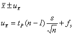
being the Student-factor, and 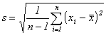designating the empirical standard-deviation. In contrast to (7), the ISO-Guide would note



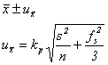
Unfortunately, the definition of the auxiliary factor is backed by no formalism. Setting , the uncertainty would clearly be too small. Switching over to the extended uncertainty of the ISO-Guide, defined by selecting , the uncertainty would make sense. However, as there is no clear mathematical way to arrive at such an uncertainty expression; not every experimenter might be happy with it.

The situation gets worse in case of error propagation.

Here we have to combine two or more measured quantities - arriving at the second of the two branching points announced: As has been shown in [5], in combining e.g. two means within a given function , it is strongly recommended to always refer to the same number of repeated measurements, . Then the overall uncertainty of is simply given by, [4,5],

(8) + .

The quantity denotes the Student-factor and the empirical variances and the empirical covariance of the measured values. To assess the unknown systematic errors





the triangle inequality has been used, [4].

Though



with

,

designates a confidence interval for with probability P, no probabilty statement should be associated with (8). Clearly, the reward coming along with (8) is the safety or better to say, the objectivity of the statement: The experimenter knowns where to locate .

We add that formula (8) may easily be extended to error propagation streching over several successive stages what, indeed, corresponds to the standard situation in metrology. Thereby the new formalisms work like a bilding kit.

In contrast to (8), the ISO-Guide specifies



where again fixes the uncertainty and the extended uncertainty.

Again, there is neither a hint nor a criterion when and why we should use one or the other uncertainty. In particular, it remains an open question, why we are limited just to - as any other value, e.g. , could also have been used.

Submitting uncertainty (8) and the - uncertainty to computer simulations, the result is smashing: While uncertainty (8) turns out to be reliable in any case, the uncertainty is completely unsatisfying. Any - value other than has not be tested - the reason being, that the concept of auxiliary - factors appears to be unfounded. At this point we should remember, that the uncertainties of the fundamental physical constants as given by CODATA are uncertainties.

After all, the author is not in a position to back the decision of the many famous international societies

BIPM International Bureau of Weights and Measures

ISO International Organisation for Standardisation

IEC International Electrotechnical Commission

IUPAC International Union of Pure and Applied Chemistry

IUPAP International Union of Pure and Applied Physics

IFCC International Federation of Clinical Chemistry

OIML International Organisation of Legal Metrology

and the National Metrological Institutions of the world to support the ISO-Guide.

Formula (8) expresses the aim of any experimenter, to run a well defined, stable experimental set-up and to investigate a well defined physical effect. To such a constellation belongs the model of a stationary statistical ensemble (each member comprising the same unknown systematic error). And if the situation is as such, we should model it as such and not according to a softening of the distiction between random and systematic errors as the ISO-Guide does.

Formula tends a bit in the direction of robust statistics (sufficiently high), which, of course, is an important concept. Should metrology needs robust statistics, it certainty would not aim at high level accuracies. This, however, is a crucial point:

Metrology lacks a reliable uncertainty concept for high level accuracies.

3.2 Method of least squares

Biased input data influence least squares significantly: Even if the variances of the input data are expected to be equal, the adjusted linear system does not yield an estimator for just that variance. Then, in particular, the most basic least-squares-tool, the Gauss-Markov-Theorem, breaks down.

To cure these effects, the adjustment should not rely on individually measured data, but on mean values, so that the associated empirical variances are known a priori. Furthermore, as there is no weighting matrix in the sense of Gauss-Markov, an empirical diagonal matrix,

(9) .

should be introduced. The variation of the elementsof G by trial and error minimizes the uncertainties of the adjusted parameters, [7].

The new error formalisms describe the couplings between the adjusted parameters as follows: With us, each of the input data comprises the same numbers of repeated measurements, consequently, Hotelling's density turns out to be applicable. This distribution is able to formalize the dependencies between the adjusted parameters due to random errors. Remarkably enough, the associated confidence ellipsoids are free from unknown theoretical variances and covariances, what should be considered a significant progress in regard to those confidence ellipsoids, used within classical error analysis. - As is well known, the latter ones are taken from the exponent of the multidimensional normal probability density, which, however, is based just on those unknown theoretical variances and covariances.

The couplings due to unknown systematic errors also lead to spatial objects, which the author has called security polytopes. Even the combination of both spatial figures, confidence ellipsoids and security polytopes, is possible, as has been shown in [6]. These figures, in a certain sense, may remind us of convex potatoes.

 

3.3 Analysis of variance

There will hardly be any empirical data being free from unknown systematic errors or biases. Admitting this fact, the much beloved tool, analysis of variance, has to be rejected once and for ever, should that be acknowledged or not.

We have to state: Unknown systematic errors, superposed to empirical data, abolish the tool analysis of variance.

Nevertheless, the new formalisms may be called upon to pairwise compare a given set of arithmetic means aiming at one and the same physical quantity. In the simplest case, let there be just two means, and . Let , then, any difference , satisfying the relation

(7)

implies compatible arithmetic means and .

4. Appropriate application of the triangle inequality

Finally, some words are in order in regard to an appropriate application of the triangle inequality or to the uniqueness of the propagation of unknown systematic errors. Of course, overall-uncertainties should be quite independent of the specific path taken, given that there is more than one. To verify this strict independence, we consider the expression



and expand

where



specifies the propagated systematic error of . An estimator for is

, .

Now we expand ,

,

where



designates the proagated systematic error of . Inserting we find

,

so that we finally arrive at the reasonable estimator

,.

In contrast to this, we would get a nonreasonably propagated systematic error, if we inserted in



the previously defined

.

This would cleary be an inconsistent action leading lastly to an unecessary overestimation.

5. Conclusion

The decision not to randomize unknown systematic errors and, in error propagation, to rely on equal numbers of repeated mesurements for each of the variables implied leads to a new kind of error calculus, yielding one dimensional uncertainty intervals and multidimensional uncertainty spaces, covering or including the true values of the pysical quantities aimed at with reasonable or common sense security.

The new formalisms work like a bilding kit, are lucid, easy to control and to check. Above all, their error budgets correspond to the basic demand of physical objectivity. In this respect they do realize the fundamental metrological concept of universal tracebility.

References

[1] ISO, Guide to the Expression of Uncertainty in Measurement, 1993. 1, Rue de Varambe, Case postale 56, CH-1211 Geneve 20, Switzereland.
The Guide ist based on the recommendation 1 (CI-1981) of the CIPM and on the recommendation INC-1(1980) of the „Working Group on the Statement of Uncertainties“ of the BIPM. It has has been signed by the ISO, IEC, IFCC, IUPAC, IUPAP and the OIML.
[2] Eisenhart, C., The Reliability of Measured Values- Part I, Fundamental Concepts; Photo-
grammetric Engineering, 18 (1952) 543-561
[3] Eisenhart, C. in H.H. Ku (Ed): Precision Measurment and Calibration, NBS Special
Publication 300, Vol 1. (US Government Printing Office), Washington D.C., 1969
[4] Grabe, M., Principles of „Metrological Statistics“, Metrologia 23 (1986/87) 213-219
[5] Grabe, M. Towards a New Standard for the Assignment of Measurment Uncertainties,
National Conference of Standard Laboratories, 31. July-4. August 1994, Chicago
[6] Grabe, M., Uncertainties, Confidence Ellipsoids and Security Polytopes in LSA, Physics Letters A 165 (1992) 124-132 - Erratum A 205 (1995) 425
[7] Grabe, M., An Alternative Algorithm for Adjusting the Fundamental Physical Constants,
Physics Letters A 213 (1996) 125-137